Normal Distribution

The Normal Distribution is the last form of distribution discussed in this course. It is itself a form of continous random variable, thus it's curve is completely undisrupted. When graphed it appears as a bell-shaped curve, something you may have heard of many times before.

This distribution has the notation of:

\(X \sim N(\mu, \sigma^2) \)

And looks like this:

Notice how equidistant points have different factors for \(\sigma\)/

Just like any other CRV, many questions may ask you to find the probability of a range of values within the distribution:

\(P(L \lt X \lt U)\):

Besides some known values that will be discussed later on, you would never need to calculate a range like this in a calc-free section unless special insight is required.

When you are required to calculate a probability range in a calc-assumed section / making use of a classpad/Computer Algebra System (CAS) supprted calculator, there are many ways to do this. Sure, you can integrate the defining function across the lower and upper limits... IF YOU'RE AN IDIOT!!! The best way to do this is to use the Methods eActivity functionality (Normal CDF).

Quantiles and Percentiles

If a certain proportion of the distribution falls below a certain number, that number is reffered to as a quantile of that proportion.

Bloody confusing, and phrased horribly. Just look at this examples to get an idea:

1) 0.9 of the distribution is below 25, 25 is the 0.9 quantile.

2) 0.2 of the distribution is below 130, 130 is the 0.2 quantile.

3) Half a distribution is less then 75. The 0.5 quantile is 75.

A percentile is the same as a quantile, only as a percentage. It is expressed as a 'th':

4) The 0.2 quantile is at most 48. 48 is the \(20^{\text{th}}\) percentile

5) The \(75^{\text{th}}\) percentile of a distribution is 92. Three quarters of the distribution is less then 92.

Known Quantiles

You may need to memorise some known values for quantiles as result of the 68-95-99.7 rule:

A normal distribution has 68% of the popuation within one standard deviation of it's mean, 95% within two standard deviations, 99.7% within three standard deviations.

\(\begin{aligned} X \sim N(\mu, \sigma^2) \\ \end{aligned} \)

\(P(\mu -\sigma \gt X \gt \mu) = 0.34 \)

\(P(\mu -\sigma \gt X \gt \mu+\sigma) = 0.68 \)

\(P(\mu +\sigma \gt X \gt \mu +2\sigma) = 0.135 \)

\(P(\mu+ 2\sigma \gt X \gt \mu +3\sigma) = 0.235 \)

Here is the formula for this distribution: YOU DO NOT NEED TO KNOW THIS!!

\(\displaystyle f(x) = \frac{1}{\sigma \sqrt{2\pi}} e^{-\frac{1}{2} \left(\frac{x-\mu}{\sigma} \right)^2 } \)

Of course, it doesn't need to be X, any variable can be assigned a normal distribution.

Keep in mind that the parameters of the normal distribution are the mean and the variance, NOT the standard deviation - a trap for young players.

6) Given \(X \sim N(8, 2^2)\), find:

Properties of Normal Distribution

1. Symmetrical about the mean \(\mu\)
2. Area of 1
3. Roughly, the distribution has a range of 3 standard deviations on either side of the mean

The Standard Normal Distribution

The standard normal distribution is a specific normal distribution that has a mean of 0 and a standard deviation of 1. It typically is assigned to the \(Z\) variable:

\(Z \sim N(0, 1^2)\)

Standard Scores (z-scores)

Here is the z-score formula:

\(\displaystyle \bbox[5px, border: 2px solid red]{z = \frac{X - \mu}{\sigma}} \)

We can see that a score (X) from a normal distribution \(N(\mu, \sigma^2)\) can be translated into the value (z) from the standard normal distribution \(N(0, 1^2)\).

A standardised score simply translates a distribution of scores with any mean and variance into another distribution with a mean of 0 and standard deviation of 1.

This is honestly pretty awesome, because it allows for each score in a large, confusing and incomprehensible distribution to be transformed into a more understandable value, that is much smaller. The new mean of the scores are 0, so now any z-score that is negative was below the mean, any that was positive was above the mean.

This has many real-world applications, often dealing with large/unlimited datasets:

• Measuring students test scores
• Measuring the height of children versus their age
• Measuring a populations blood pressure

Let's look at a case example, test scores:

7) The scores of an organic molecules test from a chemistry class has a mean of 65% and a variance of 81%:

\(X \sim N(65, 9^2)\)

The concept of z-scores can be applied in various ways. For instance, finding unknown parameters for a normal distribution.

Applications of Normal Distribution

8) A logging company is gaining interest for it's support of ecological projects that not only counter their own logging, but also provide strategic logging that betters local forests by substantially increasing the amount of sunlight that hits the forest floor; thereby ensuring future growth of ecological systems. A recent study has found that 15% of the logs are less then 4 metres whilst 8% of the logs are greater then 4.8m. Find the mean and standard deviation:

The procedure to follow for different questions varies quite alot, the trick is to locate specific evidence that helps you. I would suggest you underline it in a test. The two pieces of information we can use are the 15% and 8%, as well as the 4m and 4.8m.

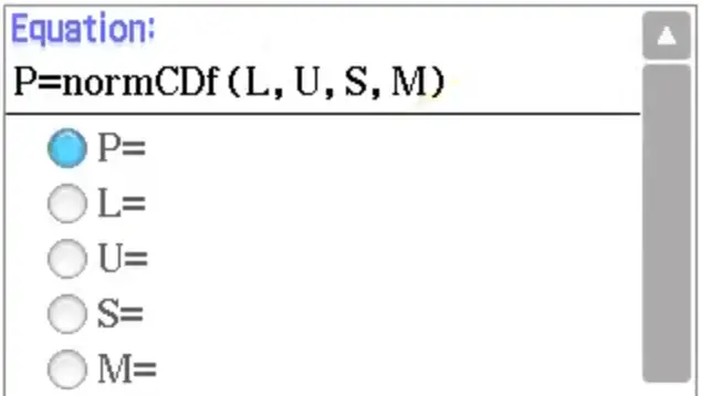
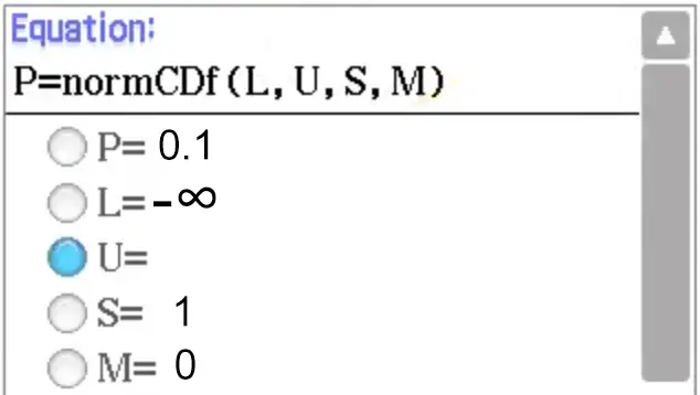
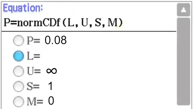
This is the key info to know: The z-score of the 4m scores is equal to the probability range of \(-\infty \ \text{to} \ U\), in which the probability is 0.1. From this information, we can calculate the upper limit using the classpad eActivity > Normal CDF (or integration... if you're an IDIOT!!! LMAO!!1). This limit IS the z-score.

To find such z-scores, navigate to eActivity > Normal CDF. This should be the menu screen:

And here is how to solve the question:

[SOLVE] >> U = -1.036

[SOLVE] >> L = 1.405

\(\displaystyle \begin{aligned} \begin{cases} -1.036 &= \frac{4+\mu}{\sigma} \\ 1.405 &= \frac{4.8+\mu}{\sigma} \end{cases} \\ \\ \mu = 4.3395 \ \ \ \sigma = 0.3277 \end{aligned} \)

9) A particular brand of light globe is normally distributed with a mean of 1120 hours and a standard deviation of 150 hours. If a globe has a life less then 675 hours, it is completely refunded.

\(\text{Let} \ X \sim N(1120, 150^2)\)

a. What is the percentage of light globes that are refunded?

\(\begin{aligned} P(X \lt 675) &= 1.505 \times {10}^{-3} \\[5pt] &= 0.151 \% \end{aligned} \)

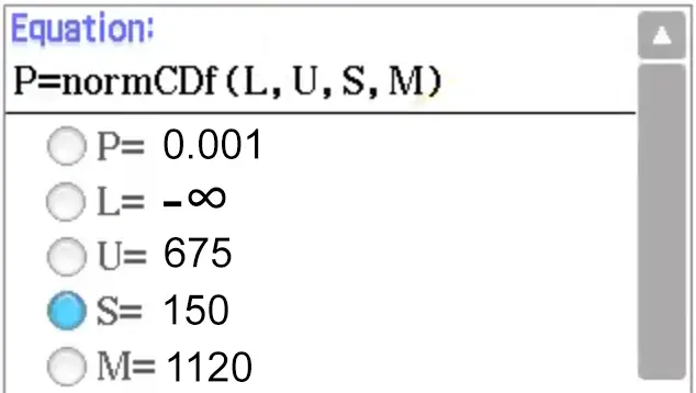
b. In an attempt to reduce the losses for the brand, the brand created a mandated policy to limit the refunded globe percentage to 0.1%. With what standard deviation is this possible?

[SOLVE]

\(s = \sigma = 144\)